
Model Documentation
This section is a technical documentation of the microWELT 3.0 model. It is organised module by module. The modules are grouped as follows:
Model Overview
The actors
The socio-demographic core
Economic activity
Labor related income
Tax-Benefit System
Health and Care
The simulation engine and associated modules
Model output
This documentation is automatically generated from the latest version of the model code.
Model Overview
MicroWELT 3.0 SUST - is a model built within the Horizon Europe SustainWELL project. It builds on the MicroWELT simulation platform, extending its scope to the modeling of longitudinal activity careers, earnings, social insurance, and tax-benefit calculation and accounting.
The model inherits most features from existing MicroWELT applications. MicroWELT is a modular, open-source modelling platform developed for the comparative study of interactions between population ageing, socio-demographic change, and welfare state regimes. MicroWELT follows a continuous-time, interacting population framework and supports the alignment of aggregate results with official population projections.The model is X-compatible, meaning it can compile source code using two programming technologies: Modgen and the new open-source environment openM++.
MicroWELT simulates three types of actors (agents): observations, persons, and an observer. ‘Observations’ correspond to records in a starting population file and are used to generate the simulated population through sampling and cloning. Observations are linked to nuclear families. They are temporary actors and are destroyed once the simulated population is created. Persons are the main units of the simulation. The single observer actor is used for processes that require aggregated information, such as model alignment.
In a nutshell, the model consists of the following components and modeled behaviors, most of which corresponding to various modules which include their own detailed documentation.
Previousely existing modules:
The simulation engine, which generates all actors known at the start of the simulation. Most importantly, it generates the initial population from a starting population microdata file.
Education, which takes into account the intergenerational transmission of education and supports trend scenarios as well as scenarios in which changes are driven by the intergenerational transmission of education.
Demography: For mortality and fertility, microWELT reproduces Eurostat’s population projections at the aggregate level, but adds detail at the individual level by taking into account variations in first birth cohort rates and resulting childlessness, progression to second births and longevity by education. Net migration is modelled on the basis of Eurostat projections by age and sex, but with the aim of keeping families together.
Partnerships are modelled from the female perspective, taking into account age, presence and age of children in the family and education. Partners are matched by assortative mating, based on distributions of age differences and education.
LTC needs, arrangements and gaps are modelled, taking into account age, gender and education, as well as the availability of a spouse and the number of children.
Model output is produced through a comprehensive set of output tables.
New modules:
Health and health status transitions used as explanatory variable in various processes, including employment, disability pensions, and mortality.
School enrolment as base of modelling the private and public consumption of education and related education benefits and family transfers.
Longitudinal activity careers distinguishing the states never active, employed, enemployed, family leave, out of labor force, retired. The model also distinguishes between full-time and part-time employment.
Earnings and earnings-replacements (4 modules), i.e. social insurance benefits connected to individual work careers such as unemployment benefits, maternity and parental leave benefits, amd pensions.
Tax-Benefit calculation (8 modules), consistent with Euromod - based on parameters derived from a synthetic tax-benefit database produced by the Euromod Hypothetical Household (HHoT) tool covering the heterogeneity of the population alongside various dimensions. The model distinguishes income taxes, social insurance contributions, and benefits grouped to family benefits, education benefits, old-age benefits, and social benefits according the National Transfer Accounting (NTA) logic.
Benefits not covered by the Euromod HHoT tool such as health benefits, housing benefits, and education grants.
Consumption distinguishing both private and public consumtion of education, health, long-term care, and all other consumtion modeled on the family and the individual level.
Longitudinal accounting of transfers including family transfers.
Childcare provided by parents (hours) and childcare arrangements.
Additional comprehensive model output is produced through an extensive set of output tables, which cover public and private transfer flows and support the comparative analysis of the operation of welfare states.
Model Actors
Observations
The Observation actor module contains the basic information that defines the Observation actor. Observatios are created as internal representations of the records in the starting population file. They are used to create Person actors of the initial simulated population, which may be smaller or larger than the initial population file. The weights of the observations are used to determine whether and how often an individual observation is represented in the simulated population. All simulated individuals have the same weight. Observation actors are temporary; once the simulated population is created, the Observation actors are destroyed to free up memory space.
In the pre-simulation phase, the file size of the starting population is determined and, based on the record weights and the size of the simulated population, the scaling factor for automatic population scaling of the simulation outputs is determined. The starting population file is a csv-file with a header row containing variable names. Both the file name and the size of the simulation are model parameters. The record layout of the starting population file is defined in this module (PERSON_MICRODATA_COLUMNS).
Variables of the starting population:
Family ID: 1234
Weight: 543.21
Time of birth: 1966 (a random number is added if the time of birth is integer)
Sex: 0 female, 1 male
Education level: 0 (ISCED 2 or lower), 1 (ISCED 3), 2 (ISCED 4), 3 (ISCED 5 or higher)
Role in family: 0 head, 1 spouse, 2 child. (The choice of head is arbitrary; in the simulation, the female partner is considered to be the head)
Currently attending school: 0 no, 1 yes
Activity status: 0 never active, 1 employed, 2 unemployed, 3 family leave, 4 out of labor force, 5 retired
Employment type: 0 not employed, 1 part-time, 2 full-time
Health limitation: 0 non, 1 limited health
Wage
Place in any wage distribution: location in the empirical residual distribution
Pension
Years worked
When the model is extended, new variables need to be added to this list. A link to the corresponding Observation is passed as a parameter to the Start function of the Person actors, so that the values of the variables can be accessed to initialise the Person actors.
Parameters:
File name** of the starting population csv file
Simulation size:** Number of simulated actors representing the initial population. In addition to the simulation size, users can also set the number of replicates (how often the simulation is repeated; run in parallel). This is done in the general scenario settings. A typical simulation size that eliminates most of the Monte Carlo variation in the aggregate results while keeping run times low (depending on computer power, ~1h) is 8 x 400,000.
Persons
The Person actor module contains the basic information that defines the Person actor. The most important function is the Start() function, which initialises all states of a person at creation. This includes initialising time. When the Start function is called (which is done by the simulation engine to create the initial population and immigrants; and by mothers giving birth) the following parameters are passed to the person:
Creation type: identifies whether a person comes from the starting population file, is an immigrant or enters by birth.
Pointer to observation: for persons created from Observations (the starting population file), this pointer allows access to the variable values from the file.
Pointer to creator: For persons created from the starting population file, this is the oldest person of the family who is created first; for births during the simulation the pointer links to the mother. It allows to access information from the the person and to establish family relationships.
Year of immigration: this parameter is only relevant for immigrants.
Sex of immigrant: this parameter is only relevant for immigrants.
After the Start function, a person is part of the simulation. At this point, immediately after birth, the “SetAliveEvent” event is called, which handles family and other actor links, and calls initialisation functions that require the person to be already in the simulation (and therefore cannot be performed in the Start function).
Observer
The Observer module contains the basic information associated with an Observer actor. A single Observer actor is instantiated in a simulation. All people are linked to the Observer at birth. The Observer is mainly used for alignment and to improve efficiency, e.g. by implementing a single year change clock instead of year change events at the individual level. At the beginning and end of each year, and in the middle of each month, clock events are called, which are used to call functions to be performed at those times. For example, at the beginning of each year the observer loops through the whole population and calls an individual level function that handles the year change, e.g. by incrementing the calendar year.
At the end of the year, just before the projected time begins, a series of initialisation functions are called. These include functions for imputing the number of children, including those not currently observed in the family, and the initial initialisation of long-term care needs and arrangements, which are then updated according to a mid-month schedule. These functions - as well as other functionalities of the Observer - are implemented and documented in the relevant modules.
Demography
Fertility
The fertility module implements births, including the imputation of past births. It is designed to simultaneously match official population projections - i.e. aggregate age-specific birth rates - and to take into account education-specific differences in age at first birth and the distribution of family sizes (0, 1, 2+ children). Family sizes are parameterised by education-specific cohort parameters, namely first birth rates by age and second birth rates by time since first birth. Children observed in the starting population are considered as own children.
First and second births that cannot be observed in the starting population because the children have already moved out are imputed, the algorithm depending on the age group:
For women aged 50+, the number of children is imputed by age and education (from a parameter). In addition, log odds are used to select women (of a given education and age) by their current partnership status. The algorithm takes into account observed children in the family, so the number of children can only increase.
Women under 36 are assumed to live with all their children, so family size is assumed to be equal to the observed number of children in the family.
Women aged 36-49: Based on first birth rates, the number of women expected to be a mother is calculated for each education group and age. This number is compared with the number of observed mothers and the gap is closed by finding suitable women who are assumed to have given birth more than 18 years ago (i.e. to children who have already moved out and therefore cannot be observed in the starting population). Once these women have been identified (as in the case of first births, the algorithm also takes into account current partnership status), the date of first birth is assigned. For the remaining time window (from the imputed first birth to 18 years before the start of the simulation), second births are assigned according to second birth rates. While this algorithm is intended to be a realistic allocation of motherhood, the number of second births so far does not take into account cases where one child is observed in the family but this child is not the first child, i.e. the first child has already moved out. To account for these cases, the probability that an observed single child actually has an older sibling is calculated and additional first births are imputed.
The fertility module focuses on women. Apart from the observed number of children from the starting population, family characteristics from the male perspective are treated in a separate module.
Within the simulation, births are modeled the following way:
Birth events are created based on age-specific period rates. The women triggering the event are not considered to be the mothers; the most likely women of similar age to give birth still has to be identified.
Events for expected first births are created by applying education and cohort-specific first birth rates. Women expecting a first birth are given first priority to become the mothers of the babies created by the birth events. Applying age-sepcific first birth rates implicitly determines education-specific cohort childlessness.
Events for expecting a second birth are created by applying education and cohort specific second birth rates. Women expecting a second birth are prioritised to become the mothers of the babies created by the birth events if no woman expects a first birth.
Higher order births are randomly assigned to women of the given age who already have two or more children.
Parameters:
Age-specific fertility rates: this parameter is usually taken from official population projections. As explained above, it is used as an adjustment target, creating birth events without deciding which woman of the given age will be the mother of the child.
First birth cohort rates by education: This (age-specific) parameter - available e.g. from the Human Fertility Database - is used to model ‘expected’ first births. The parameter is also used to impute past births that cannot be observed in the starting population because the children have already moved out. As the required cohort data are only available for the past and are age-censored for cohorts that have not yet reached the end of their reproductive life, the parameterisation requires scenario assumptions.
Duration-specific parity progression to second child by education: This parameter is used to model ‘expected’ second births by time since first birth. The parameter is also used to impute past births that cannot be observed in the starting population because the children have already moved out. Obtaining this parameter typically involves estimation from survey data and calibration to scenario-based projections of education-specific parity progressions.
Distribution of number of children by age and education for women aged 50+. This parameter is used to impute family size. It is usually obtained from retrospective information collected in survey data such as SHARE.
Odds ratio of having at least one child comparing women in a couple with single women by age group. This parameter is used to impute family size to women aged 50 and over. It is usually estimated from retrospective information collected in survey data such as SHARE.
Odds ratios of having two or more children comparing mothers in a partnership with mothers not currently in a partnership, by age group. This parameter is used to impute family size to women aged 50 and over. It is usually estimated from retrospective information collected in survey data such as SHARE.
Mortality
The mortality module implements mortality by age, sex, education and health. It is designed for cases where mortality projections taking into account educational differences are not readily available, but have to be derived by combining information from (1) official population projections with (2) data and scenarios on remaining life expectancy at ages 25 and 65 by education and (3) age-specific mortality differences (relative risks) by education observed today. In terms of educational attainment, this module distinguishes between three levels: low (ISCED 2 and below), medium (ISCED 3 and 4) and high (ISCED 5 and above). Health status is accounted for in a final step, drawing on the health transition model.
Users have three choices of how to simulate mortality:
Base model: This option does not model mortality by education and health, but simply applies aggregate period mortality rates by age and sex (typically taken from official population projections).
Detailed model: This option models mortality by education using target remaining life expectancies at ages 25 and 65 and relative risk profiles from parameters. For each year and level of education, the period mortality rates of the base model are calibrated to produce education-specific period life tables. (This step is performed in the pre-simulation function of this module). In the final step, once the age, sex and education of the next person to die have been determined, the person with the shortest waiting time, accounting for health status, is chosen from the pool of people with these characteristics.
Detailed model adjusted to base model total mortality: This option additionally adjusts mortality by age and sex to the base model. This means that mortality projections taken from official population projections are reproduced in aggregate (by age and sex), while maintaining the relative risk structure between education and health groups.
In order to construct education-specific life tables, two calibration factors by education level (applied together with the age patterns in relative risks) are determined by numerical simulation (binary search). First, a calibration factor is sought to fit the remaining life expectancy at age 65. Second, using this factor for the 65+ population, another calibration factor is determined for the younger ages to fit the remaining life expectancy at age 25. As relative risks by education usually have an age shape (relative differences typically decrease with age), the calibration factors are applied together with the parameter of current age-specific relative risks. In other words, individual mortality is calculated by applying the relative risk factor - rescaled by the calibration factors - to the mortality rate by age and sex taken from official population projections. The underlying assumption is that age patterns in relative risks remain the same over time. For the starting year, this approach is consistent with the direct application of life tables by education (as far as the remaining life expectancies in the parameters are consistent with these life tables), so no calibration is required at the start.
The parameterisation allows the creation of scenarios for the evolution of educational differences in life expectancy, such as convergence scenarios where the gaps between groups narrow or close.
The third model option allows for an additional adjustment of the results of the education-specific model to the aggregate mortality of the base model. This adjustment preserves the relative differences in mortality risks by education. It is implemented by separating the birth events by age and sex produced by the base model from the selection of those selected to die, the latter being based on individual random waiting times taking education into account. Statistically, this approach is equivalent to modifying the baseline mortality hazard (but maintaining the relative risks by education) in such a way that, for a given composition of the population by education, the overall mortality rate is equal to the target mortality rate.
Parameters:
Model option: allows the user to choose between the three model options described above.
Period mortality by age and sex: this parameter is usually taken from official population projections.
Remaining life expectancy at ages 25 and 65 by education, sex and period. Recent estimates are available in the literature and/or can be calculated from period mortality rates by age, sex, and education. The parameter allows the construction of scenarios on the evolution of educational differences, e.g. concergence scenarios.
Current age-specific relative mortality risks by education and sex. This parameter can be calculated by comparing mortality rates by age, sex and education with mortality rates by age and sex. The parameter is used to capture the age patterns in relative risks, but - due the model alignments described above - does not affect education-specific life expectancies.
Migration
The migration module handles net migration by age and sex, parameters typically taken from official (e.g. Eurostat) population projections. Immigrants are created by the simulation engine, their number and age distribution being calculated from the net migration parameter in the pre-simulation function in this module. Immigrants arrive at random times within a year. In contrast, emigration is modelled as occurring only once in the middle of each year. Emigration is handled by the Observer actor, the event implemented in this module. The migration module also initialises the educational and family characteristics of migrants and links migrant mothers to children arriving in the same year. The concept of net migration does not allow for the modelling of life course heterogeneity by place of origin, so immigrants are assumed to be no different from residents.
Like all other persons, immigrants are created at birth. Unlike residents, they are not subject to life course events such as mating or mortality until they immigrate. Instead, they acquire most of their characteristics by cloning from a resident host. This happens at two points in time:
At birth, babies sample their educational ‘destiny’ and their parents’ education from resident babies.
At the time of immigration, a resident host of the same age, sex and education is randomly selected and relevant characteristics are cloned. For women, this includes characteristics such as number of children and whether a first or second birth is currently expected. If a female host lives with dependent children, the corresponding female immigrant tries to find children of the same age in the pool of immigrants arriving in the same year (so far unattended). While this approach treats the fertility of immigrant women as similar to that of the resident population, it does not treat partnerships separately. All immigrants arrive as singles (including single mothers with dependent children) and, from the next mid-month event onwards, become subject to the periodic partnership updates treated in the partnerships module.
Parameters:
Migration On/Off
Number of net migrants by age, sex, and year
Family
Partnerships
This module implements processes for maintaining the partnership status of women over the life course (union formation, dissolution, matching a suitable partner). The female partnership status is updated monthly according to observed partnership patterns by education, age, and age of the youngest child.
The model maintains the patterns contained in the parameters. Thus we assume that these patterns are stable and changes in aggregate partnership characteristics only result from compositional changes in the female population like changes in the education composition, childlessness or timing of births. The model follows a ‘minimum necessary corrections’ approach changing the union status of women only to meet aggregate numbers. In reality, unions are more unstable, i.e. the model does not move women out of a union and others in if the aggregate proportion does not change. The current version is longitudinally consistent only on the cohort level by education and the number of children ever born (childless, one child, two or more children). Alignments can be switched off for higher ages (see below).
Partner matching is modelled by age and education. We model only two-sex couples. For age differences, we assume that the patterns of observed age differences in couples by age persist over time. One difficulty in assigning a partner is that the distribution of age differences changes with age at union formation. For example, a young man cannot have a much younger spouse (or vice versa), while the spread of observed age differences increases with age. As information on union formation and duration is usually not available in surveys and administrative data are only available for marriages, we follow an indirect approach based on the observed age patterns in existing partnerships. The algorithm is as follows:
Based on the distribution parameter of age differences between spouses, we calculate the expected number of partners by age for the age of the seeking woman in the simulation.
We then calculate the number of actual partners by age in the simulated population.
By comparing the expected and observed distributions, we identify the age with the largest negative gap for which there is at least one available male partner.
Having identified the pool of available partners, a second criterion is education, which is sampled from a distributional parameter. Current patterns are assumed to be persistent and maintainable over time. Although the model is female-driven, the number of men available for partnerships can be limited by setting parameters for the maximum proportion of men in partnerships according to age group and level of education. This prevents changes in the educational composition (e.g. a diminishing proportion of men in the lowest education group) from causing unrealistic changes in the likelihood of men being in a partnership according to their education level (e.g. all men in the lowest education group being in partnerships).
Parameters:
Partnerships of women with dependent children: probability of being in a partnership by education, age group and age group of youngest child. This parameter is usually estimated from survey data such as SILC. These probabilities are assumed to remain constant in the future.
Partnerships of women not living with dependent children: probability of being in a partnership by education and age. This parameter is usually estimated from survey data such as SILC. These probabilities are assumed to remain constant in the future.
Highest age at union dissolution other than widowhood: This parameter makes it possible to switch off the adjustment to (lower) target rates. This is useful for creating scenarios that assume union stability at higher ages, where, due to improvements in mortality, it can be assumed that people stay in unions longer because of the increase in life expectancy of the partner.
Highest age at union formation: This parameter allows to switch off the adjustment to (higher) target rates. This is useful for sensitivity analysis, i.e. to create scenarios in which no new union formation occurs from a certain age.
Option to adjust the union status of persons of the staring population to the target parameters before the start of a simulation. This enables identical initial partnership patterns to be created for scenario comparisons with scenarios that restrict the age of union adjustments.
Union formation risks 65+: this parameter allows to generate scenarios, which combine the assumption of union stability at ages 65+ together with new union formations
Distribution of partner ages by age of female partner: This parameter is usually estimated from survey data such as SILC. It is assumed that these distributions will remain constant in the future.
Distribution of partner’s education by education level of female partner. This parameter is usually based on educational patterns of currently young couples, estimated from survey data such as SILC, It is assumed that these distributions will remain constant in the future.
The maximum proportion of men available as spouses by age group and education.
Family
The family module manages and maintains family relationships. MicroWELT is based on the concept of nuclear families, where a family consists of a household head, a spouse (if present) and dependent children. Accordingly, each person has a family role: head, spouse or child. The female spouse is considered to be the head of the family. The model distinguishes between four types of family link:
Links between spouses, maintained over the simulation and dissolved upon union dissolution;
Links to ‘first’ parents (biological or the first known mothers and fathers, as observed in the starting population) are maintained for as long as the parents are alive.
Links to the ‘most recent’ parents (e.g. stepparents). These links are maintained as long as the ‘most recent’ parents are alive.
Links to cohabiting parents: these are the ‘most recent’ parents as long as children stay at home. The link is dissolved when the children move out.
The module contains a collection of functions that handle links at specific life history events:
Death: If there is no spouse but children in the family, each child checks whether it has a biological mother or father or a grandmother or grandfather still alive, in which case the child links to a new guardian (and - if present - to the spouse of this new social parent).
Partnerip formation: Partners are linked and form a new nuclear family. All children update their family links.
Dissolution of the union: Before the union between partners is dissolved, all children have to choose with whom they want to live. The choice is modelled by a set of simple rules and a probability to stay with the mother. If only one of the two parents is a biological parent, the children choose to stay with the biological parent. Otherwise, the choice is random, depending on the probability parameter.
Initial family ties of persons in the initial population: Links between spouses and to mothers and fathers; the observed parents are assumed to be the ‘first’ as well as the ‘recent’ parents.
Parameters:
Probability of living with mother after dissolution of parental partnership
Family from the male perspectice
The modelling of family formation and dissolution in microWELT is female-driven, with males selected by assortative mating, taking into account age and education. Accordingly, male parity is updated with the birth of children by a partner. As only current partnerships and dependent children in the household can be observed in the starting population, information on other children is missing. This is taken into account by the following assumptions and approaches:
For men in the starting population living in a partnership, they are assumed to have the same number of children as their partner. This includes the imputed information on the number of children modelled in the fertility module (children who have already left home).
Male childlessness by education is modelled by a cohort parameter. To achieve this target childlessness, at the start of the simulation a proportion of currently childless men are flagged as never becoming fathers. If they become parents during the simulation, the flag is passed on to an unflagged childless man of the same age and education. During the simulation, flags are set at birth.
Single men aged 65+ at the start of the simulation who are not flagged as never becoming fathers are assumed to be fathers. Similarly, men who are not flagged as never becoming fathers when they turn 65 in the simulation are assumed to be fathers. This addresses a potential mismatch between the female-driven family dynamics and the male childlessness parameter and should affect only few people in the simulation. (No such correction is made if too many men are fathers at age 65 relative to the childlessness parameter). In all these cases of imputed fatherhood, the number of children (one versus 2 and more) is randomly decided on the basis of a parameter for the parity progression to the second child.
Parameters:
Male cohort childlessness by education
Male parity progression to second child used for imputation
Leaving Home
The Leaving Home module deals with the economic emancipation of children. In the current model, children leave home at the age of 18, when they form their own nuclear family due to union formation a/o parenthood.
Education
Parents Education
Parental education is used to model the intergenerational transmission of education. It refers to the highest educational attainment of both parents. Parental education can be at one of three levels - low (ISCED 2 and below), medium (ISCED 3 and 4), high (ISCED 5 and above) - or unknown. Modelling the educational ‘destiny’ of a child requires knowledge of the educational composition of the parents of the child’s birth cohort, as odds ratios based on parental education need to be taken into account, while at the same time meeting outcome targets regarding the educational distribution of the child’s birth cohort.
Parental education is initialised at birth. Information on the current educational distribution of parents is provided by an observer function that tracks and allows retrieval of this distribution information based on the past 12 months, updated at each birth.
Education
The education module decides the highest education attained by a person accounting for gender, year of birth, and parents’ education. The individual educational “destiny” is decided at birth. Gender and cohort specific outcome distributions can be specified by parameters. In addition, the model allows the specification of relative differences in educational attainment by parental education (intergenerational transmission of education, parameterised by odds ratios). In this way, for a given cohort’s educational distribution, parental background is taken into account when deciding who will receive which education. This alignment to cohort targets can also be switched off from a given point in time, after which educational change is driven entirely by the changing educational composition of the parents’ generation. For individuals in the initial population, the educational information on attendance and attainment from the starting population file is respected:
Older cohorts (born before 1990; the cut-off is set in the Context module) retain the same education as in the starting population.
Younger cohorts (born after 2000; the cut-off is set in the Context module) have their educational trajectories (re)assigned on the basis of the model parameters.
For intermediate cohorts, educational information from the starting population (school attendance, current highest level of education) is used, but higher levels of education can still be achieved by those who are enrolled in education. The model attempts to simultaneously respect the information from the starting population and meet the cohort targets set in the parameters. This is achieved through a combination of sampling and storage/retrieval of educational attainment. If a sampled education does not match the individual’s starting population information, it is stored in an array maintained by the observer and sampling is repeated. If the array is not empty, persons first check whether it contains an educational outcome that matches the individual characteristics of the starting population record.
Within the simulation, information on educational outcome targets and relative differences by parental education, together with the educational composition of parents, is used to determine individual progression rates consistent with the targets. This is achieved by numerical simulation (binary search for base odds which, when combined with odds ratios by parental education, give the target probabilities for the parental education distribution at that point in time). The distribution of parental education is derived within the simulation on the basis of births in the last 12 months. The information on births by parental education and month is maintained by the observer.
Parameters:
The distribution of educational attainment (4 levels) by cohort and gender. The levels are ISCED 2 or lower, ISCED 3, ISCED 4, and ISCED 5 or higher.
Odds ratios by sex and parental education (3 levels; ISCED 3 and 4 are combined) for each transition between school levels.
The (first) year from which educational attainment by gender and parental education is fixed. This parameter makes it possible to switch off the adjustment of outcomes to the distribution of outcomes and to model the change in education entirely as a result of the changing composition of parental education.
Education Enrolment
This module handles educational enrolment based on the enrolment patterns observed in the initial population. It is assumed that the age-specific enrolment rates will remain as they are today for a given educational outcome. This means that the dynamics are entirely driven by composition effects due to educational expansion. The enrolment rates used in the simulation are implemented as a state of the observer actor, which is initialised by the InitializeEnrolmentAtStart() function. This function is called before the simulation starts, once the educational fate of all members of the initial population has been determined based on their highest level of education, enrolment status, parental education, and expected cohort outcomes as defined in the scenario parameters.
Economic activity
Activity Transitions
This module implements economic activity status and longitudinal activity transitions. In terms of economic activity, the model distinguishes between:
Never active
Employed
Unemployed
Family leave
Out of labor force
Retired
The module incorporates longitudinal, consistent employment careers modelled in continuous time. Transitions between labour market states depend on a set of personal characteristics such as gender, age, and education as well as the duration in the respective state. Most transitions are based on piecewise constant hazard regression models:
Employed -> unemployed
Employed -> out
Unemployed -> employed
Unemployed -> out
Out -> employed
Out -> unemployed
Unemployment can be aligned to a (logistic) model of the prevalence of unemployment by individual characteristics. Such an alignment can be used to create scenarios that close gaps between groups, for example by improving employment opportunities for the elderly workforce or people with health limitations. Additionally, in a second step, total outcomes can be aligned to an overall unemployment rate (a scenario parameter). The alignment routine modifies the process from employment to unemployment, determining the proportion of the work-force, grouped by gender, education, age and health, affected by unemployment. Within each group, the selection of individuals who become unemployed is still determined by their individual transition hazards.
In the same way, labor force participation can optionally be aligned to a (logistic) model of the labor force participation (prevalence) by individual characteristics. Such an alignment can be used to create scenarios that close gaps between groups, for example by increasing labor force participation of the elderly, of people with health limitations, or women. The alignment routine modifies the process of leving the work-foerce from employment and unemployment, determining the target proportion of people in the labor force grouped by gender, education, age, health, and the age of the youngest child. Within each group, the selection of individuals who exit the labor force is still determined by their individual transition hazards.
The initial state durations are determined by sampling simulated duration spells created within the simulation. Donor characteristics are produced using the transition models that drive activity careers already in the past. Sampling occurs slightly more than two years before the simulation actually begins, since the longest duration spell is two years or more. Based on these sampled duration spells, transitions to the current state observed in the starting population are scheduled in the past.
First entry into the labor-force is modeled by entry hazards by age, gender and education. Retirement is modelled by applying a set of rules which determine, if a person leaving the work-force is assumed to permanently retire.
Parameters:
Activity transitions: collection of hazard regressions
First entry into the labour-force: hazards by gender and education group
Unemployment alignment options: no alignment. Alignment to prevalence scenario. Additional alignment to overall rates.
Probability of unemployment: logistic regression coefficients - used for optional alignment and for scenarios
Unemployment alignment targets: overall rates by year
Labor force participation alignment options: no alignment. Alignment to prevalence scenario.
Probability of labor force participation: logistic regression coefficients - used for optional alignment and for scenarios
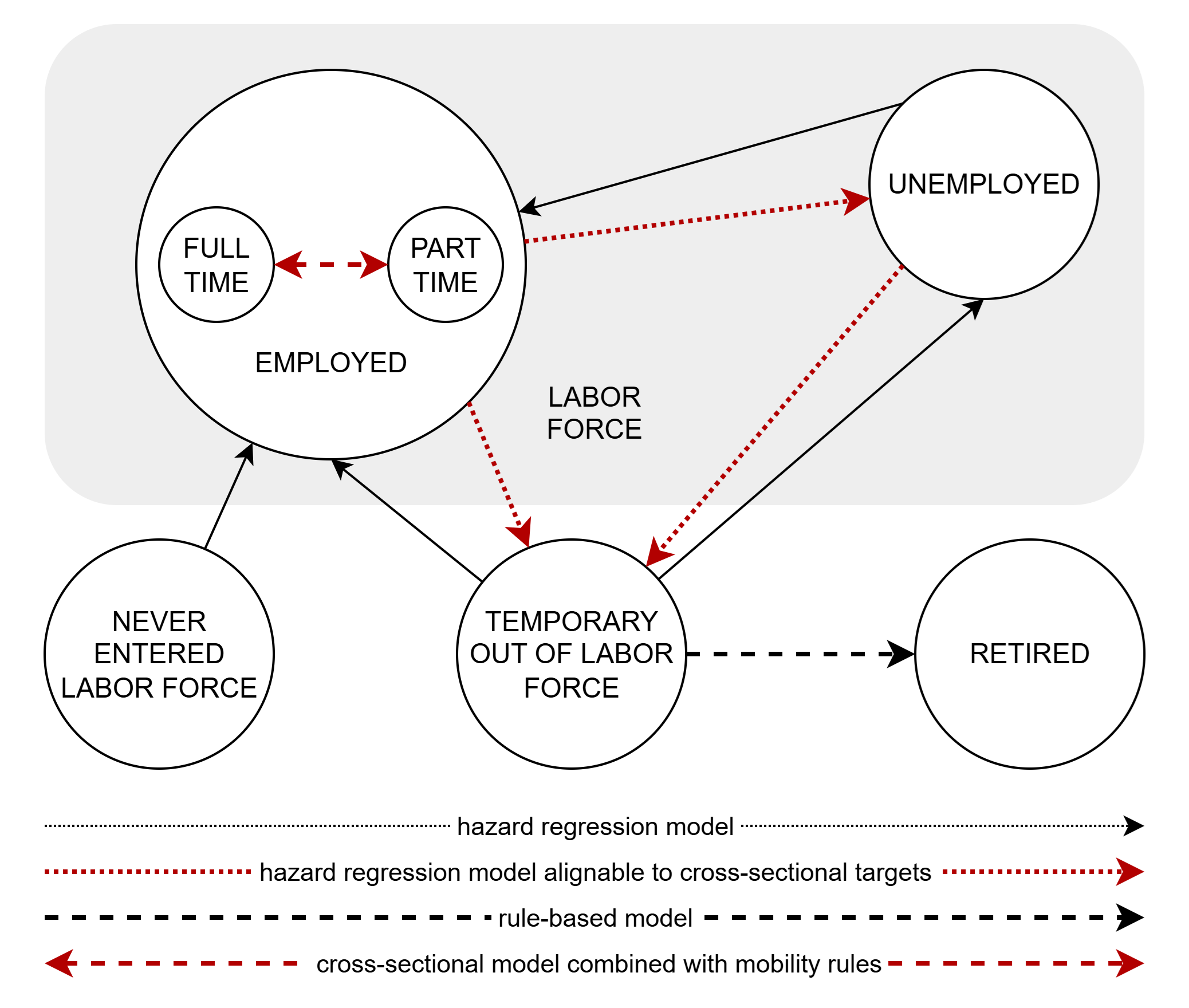
Part-time Work
This module covers part-time work. The probability of part-time employment is calculated using logistic regression and takes into account gender, the presence of children in the family and their age, education level and age. The status is updated when new employment is entered and maintained monthly. As people tend to remain in the same status for extended periods rather than switching between statuses, the model aims to keep people in their current status while simultaneously meeting the modelled probabilities based on individual characteristics. As no longitudinal data are available for modelling full-time to part-time transitions, we apply an experimental approach. People are grouped into 50 part-time risk quantiles. Each month, a new preliminary state is assigned, and individuals scheduled to change their status are identified and flagged. Next, actors try to find another person within the same risk group who has been flagged for a transition in the opposite direction. If they find someone, both individuals’ transitions are cancelled. If they do not find someone, their status changes. Mobility between states can be increased by a parameter that determines the probability that an actor will try to remain in the current state.
Parameters:
Probability of part-time work: coefficients from logistic regression
Mobility between full-time and part-time states: Probability an actor tries to remain in the current state
Tax-Benefit System
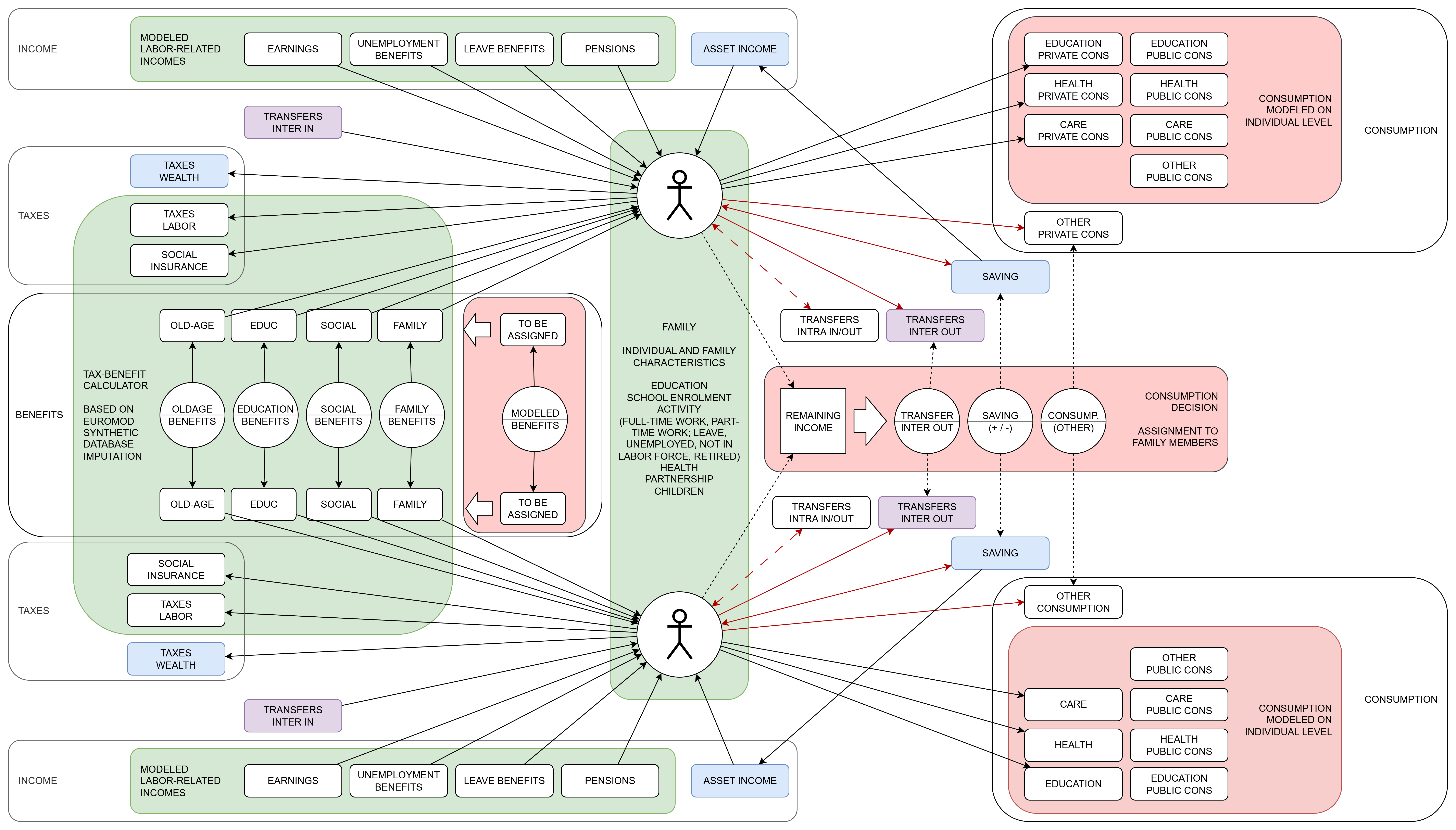
Tax-Benefit General
This module implements general tax- and benefit-related functionalities that are not specific to any particular taxes or benefits. These include a set of states that define family types and income categories, which are used as inputs for tax and benefit calculations.
Tax-Benefit Accounts
This module implements individual accounts. Currently (the list will be expanded as additional transfers etc. become available) people store yearly totals of:
Earnings
Unemployment benefits
Parental leave benefits
Public pensions
Own social insurance contributions
Social insurance employer contributions
Income tax
Old-age benefits
Family benefits
Education benefits
Social benefits
These accounts are used for lifetime accounting, such as calculating the present value of transfers. Updates are performed at the end of each calendar year, as well as upon death or emigration. The calculation of amounts is based on continuous time updates of the respective variable (such as earnings), thus adapting to all changes throughout the year.
Income Tax
This module implements income taxes on earnings and earning-related incomes (pensions, leave benefits, unemployment benefits) based on parameter tables created using the Euromod Hypothetical Household Tool (HHoT). These tables are multidimensional by family type and fine-grained income categories of earnings, unemployment benefits, pensions, and maternity and parental leave. Family types were created by accounting for partnership status and family composition according to the number and age of children. There are separate parameters for singles and couples, combined with four income types for both partners. For instance, the parameter ‘Income tax couple employed x unemployed’ applies to couples where the person is employed and has an unemployed spouse. Income taxes are calculated at the indicidual level. Taxes are updated in continuouse time whenever the tax base changes.
Parameters:
Income tax single employed
Income tax single parental
Income tax single retired
Income tax single unemployed
Income tax couple employed x employed
Income tax couple employed x unemployed
Income tax couple employed x parental
Income tax couple employed x pension
Income tax couple employed x out
Income tax couple unemployed x employed
Income tax couple unemployed x unemployed
Income tax couple unemployed x parental
Income tax couple unemployed x pension
Income tax couple unemployed x out
Income tax couple parental x employed
Income tax couple parental x unemployed
Income tax couple parental x pension
Income tax couple parental x out
Income tax couple pension x employed
Income tax couple pension x unemployed
Income tax couple pension x parental
Income tax couple pension x pension
Income tax couple pension x out
Education Benefits
This module implements education benefits based on parameter tables created using the Euromod Hypothetical Household Tool (HHoT). These tables are multidimensional by family type and fine-grained income categories of earnings, unemployment benefits, pensions, and maternity and parental leave. Family types were created by accounting for partnership status and family composition according to the number and age of children, resulting in 35 types in total. There are separate parameters for singles and couples, combined with four income types for both partners. For instance, the parameter ‘Education benefit couple employed x unemployed’ applies to couples where one partner is employed and the other is unemployed. Benefit amounts are retrieved on the family level and distributed by the family head to children in education. Benefits are updated monthly.
Parameters:
Education benefit single employed
Education benefit single parental
Education benefit single retired
Education benefit single unemployed
Education benefit single out
Education benefit couple employed x employed
Education benefit couple employed x unemployed
Education benefit couple employed x parental
Education benefit couple employed x pension
Education benefit couple employed x out
Education benefit couple unemployed x unemployed
Education benefit couple unemployed x parental
Education benefit couple unemployed x pension
Education benefit couple unemployed x out
Education benefit couple parental x pension
Education benefit couple parental x out
Education benefit couple pension x pension
Education benefit couple pension x out
Education benefit couple out x out
Family Benefits
This module implements family benefits based on parameter tables created using the Euromod Hypothetical Household Tool (HHoT). These tables are multidimensional by family type and fine-grained income categories of earnings, unemployment benefits, pensions, and maternity and parental leave. Family types were created by accounting for partnership status and family composition according to the number and age of children. There are separate parameters for singles and couples, combined with four income types for both partners. For instance, the parameter ‘Family benefit couple employed x unemployed’ applies to couples where one partner is employed and the other is unemployed. Benefit amounts are retrieved on the family level and distributed by the family head to children. Benefits are updated monthly.
Parameters:
Family benefit single employed
Family benefit single parental
Family benefit single retired
Family benefit single unemployed
Family benefit single out
Family benefit couple employed x employed
Family benefit couple employed x unemployed
Family benefit couple employed x parental
Family benefit couple employed x pension
Family benefit couple employed x out
Family benefit couple unemployed x unemployed
Family benefit couple unemployed x parental
Family benefit couple unemployed x pension
Family benefit couple unemployed x out
Family benefit couple parental x pension
Family benefit couple parental x out
Family benefit couple pension x pension
Family benefit couple pension x out
Family benefit couple out x out
Old-Age Benefits
This module implements old-age benefits based on parameter tables created using the Euromod Hypothetical Household Tool (HHoT). These tables are multidimensional, categorising families by type and income from earnings, unemployment benefits, pensions, and maternity and parental leave benefits. In order to receive old-age benefits, at least one person in the family must be retired. Family types are determined by partnership status and family composition according to the number of children. Separate parameters apply to singles and couples, combined with four income types for both partners. For example, the parameter ‘Old-age benefit: couple pension x out’ applies to couples where one partner is retired and the other is not in the labour force. Benefit amounts are calculated at family level and distributed by the family head to spouses in a way that aims to equalise incomes. Benefits are updated monthly.
Parameters:
Oldage benefit single retired
Oldage benefit couple pension x employed
Oldage benefit couple pension x unemployed
Oldage benefit couple pension x parental
Oldage benefit couple pension x out
Oldage benefit couple pension x pension
Health and Care
Long-Term Care Hours and Mix
This module implements long-term care needs, hours and care arrangements for people aged 65+ using a comparative approach described in detail in the technical paper Comparative Modelling of Long-Term Care in Hours. This novel approach generalises an Austrian administrative procedure for assessing care needs and uses data from the Survey of Health, Ageing and Retirement in Europe (SHARE) to quantify the demand for and supply of long-term care in hours, distinguishing between
Care provided in nursing homes
Formal home care
Informal care by spouses
Other informal care
Care gap
The model takes into account a wide range of factors that influence care needs and arrangements, including age, gender, education, the presence of a spouse able to provide care and the number of children. Compared to a macro approach based on age and gender, future care needs and demand, in particular for formal care and nursing homes, are mitigated by the expansion of education (better educated people tend to need less long-term care later in life), the modelling of partnerships (improvements in longevity increase the likelihood of living with a partner) and the consideration of mortality differences by education.
In the baseline scenario, needs and care arrangements are modelled based on individual and family characteristics “as of today”, with care provision adapting to current LTC patterns. The model includes scenario support that considers different dimensions of the drivers of future change.
Constrained supply scenarios: Users can set a growth path for the supply of care, including restrictions on the supply of nursing homes (compared to current places), restrictions on formal home care services (compared to current supply in hours), and restrictions on informal care provided by others other than spouses (typically children; the growth path is applied to the hours that would be available using current supply patterns).
Demographic scenarios, such as changes in mortality assumptions or partnership status.
Scenarios of changing care needs, such as “morbidity compression”, which assumes that improvements in longevity slow the age-related process of LTC needs. Such scenarios modify the individual age applied in the LTC models.
Scenarios involving compositional effects, such as the effect of educational expansion. This is realised by allowing education effects to be switched off (equivalent to applying current age-specific patterns) or by allowing convergence towards the patterns of the highest educated group. Education scenarios modify the individual education variable entering the LTC models.
The LTC module follows a cross-sectional imputation approach with monthly updates. The regression models are based on SHARE data with hours of care needs being imputed applying administrative procedures based on limitations in Activities of Daily Living (ADL) and limitations in Instrumental Activities of Daily Living (IADL) and other related variables available in the SHARE data. Within the simulation, each monthly update follows the following steps:
LTC Needs Assessment Step 1: Determine whether a person has care needs based on current prevalence by age, sex and education. Parameters are estimated using logistic regression.
LTC Needs Assessment Step 2: Determination of hours of care from distribution tables based on age, gender and education. Parameters estimated by quantile regression.
Nursing Homes: Probability of being in a nursing home based on current prevalence by age, intensity of need, availability of a spouse capable of providing care (not having own care needs above a threshold) and number of children. Parameters are estimated using logistic regression. If the scenario does not restrict/set the supply of nursing home care, these individual probabilities are used directly. If the supply is set by the user, the individual probabilities are converted into random waiting times that are used to rank people, and the ranking is then used to allocate available nursing home places.
LTC Mix Step 1: Probability of receiving (any) home care for people not living in a nursing home and not having a spouse able to provide care. If no care is received, the hours needed are recorded as a care gap. For persons with a spouse able to provide care, it is implicitly assumed that some care is received. This follows the logic of the SHARE survey, which does not quantify care gaps when a spouse is present.
LTC Mix Step 2: Determination of the provisional (“as of today”) home care mix if home care is received. Individuals are grouped according to the intensity of their care needs, the presence of a spouse capable of providing care, and the number of children. Within each group, the same (average) care mix is applied. The care mix distinguishes between formal care at home, informal care by a spouse, other informal care and a care gap.
LTC Mix Step 3: Determination of available care. With the exception of the calculation of the supply of care available from others when current patterns are applied (a parameter of average hours provided by age and gender), this step is scenario-based. It adds up the ‘provisional’ hours by type of home-care and compares them with the available supply of care for each type for which the given scenario sets/limits the supply. For each type of care, the proportion of demand met by supply is calculated. This step is skipped if there are no restrictions on the supply of care. If supply is restricted/fixed by the user, the provisional demand is adjusted and for each care type, the hours not met by the given supply are recorded. Similarly, oversupply is recorded. In the case of care gaps due to limited supply, it is determined whether there is a spouse who is potentially able to cover these hours. This information is recorded, but no assumptions are made about whether and how gaps are closed.
Key characteristics available for model output include hours of care needed and care mix, which distinguishes different types of potential care gaps:
Nursing homes: Hours provided; number of people in nursing homes
- Formal home care:
Hours met by current provision
Hours not covered by current supply (care gap due to supply constraints)
Hours exceeding current demand and available to fill gaps in care
- Hours of informal home-care provided by someone other than the spouse
Hours met by current supply patterns
Hours not covered by current supply patterns (care gap due to supply constraints)
Hours above current demand and available to fill care gaps
- Hours of informal home-care provided by spouse
Hours meeting current patterns
Potential additional hours to close gaps due to supply constraints in formal home care and informal care by others
- Care gap
Initial gap based on current patterns (people receiving no or insufficient care)
Additional gaps (or available additional supply) due to supply scenarios as listed above
Potential additional hours provided by spouses as listed above
Care hours by type of care are accumulated over the life course. Although the cross-sectional imputation approach does not allow a detailed longitudinal analysis of distributions, it is possible to compare average hours by care type for population groups distinguished by characteristics such as birth cohort, sex, number of children, partnership status at age 65 and education.
Model parameters:
Prevalence of having LTC needs (any hours) by sex, age, and education
Decile means of LTC hours needed by persons with care needs, by sex, age, and education
Nursing home prevalence by sex, partnership status, number of children, age group, and hours needed
Probability of receiving any home care among persons not in a nursing home and not having a partner able to provide care, by need in hours and number of children
Home care mix of persons not in a nursing home: mix as shares of hours by category, by partnership status, number of children, and LTC needs in hours
Average hours of informal care provided to persons aged 65 and over (excluding spouses), by age and sex
All parameters are estimated from SHARE data as described in detail in the technical report Comparative Modelling of Long-Term Care in Hours
Scenario parameters:
Slower ageing: parameters that allow the ageing process to be manipulated. Users can set a starting age from which the rate of ageing is changed; a second parameter sets the new length of each year. This allows individual ageing to be stretched, assuming that due to improvements in mortality, care needs and care hours increase more slowly with age. For example, the parameter can be set so that a person aged 65 will age 4 years in 5 years. A person aged 70 will then be 69, a person aged 75 will be 73… and 90 will be the new 85, thus adjusting age to increasing life expectancy.
Turn off the effects of educational composition: In this scenario, the composition of education by age and sex is held constant, which is equivalent to modelling care needs in hours without taking education into account. This scenario mimics a model that does not account for educational differences. Compared to other scenarios, it quantifies the compositional effect of educational improvements.
Matching LTC to supply: on/off switch by LTC type
LTC supply: future supply by LTC type and calendar year (current supply = 1.0)
Convergence of LTC needs with those of people with the highest level of education Convergence path by calendar year (0.0 - 1.0; 0.0 if no convergence). This provides an alternative to a ‘slower ageing’ scenario, assuming that the lower LTC needs of the better educated are determined by behaviours that can and will be adapted by others.

Health Status
This module implements a binary health status, as well as health transitions between good and bad health and to death. The explanatory variables are age, sex and education. Death probabilities from the health transition parameter are used indirectely by the Mortality module to account for health status once the age, sex and education of the next person to die have been determined. (This module maintaines the information of which person has the shortest random waiting time to death from the pool of individuals with these characteristics.) While deaths occur in continuous time, the health status of all surviving individuals is updated yearly on their birthday. The initial health status of people from the starting population is read from the starting population file.
Parameters:
Age-specific health transition probabilities by initial health status, sex and education level. These probabilities refer to three possible outcomes: good health, poor health and death.
Childcare hours by parents
Childcare in minutes provided by parent(s)
Model Output
Demography
Demographic tables include tables of the projected population by age, sex and education, tables of demographic events such as births and deaths, and detailed tables on fertility and migration.
Education
Education tables present simulation outputs concerning both own and parents’ education.
Family
Families tables provide output concerning family sizes and other family characteristics.
Long-Term Care
The LTC tables provide a rich output on LTC needs in hours and the mix of care received by those in need of care. Results are presented from both a period and a longitudinal perspective, the latter accumulating LTC hours by type of care over the life course by birth cohort, sex and education.
Validation
Validation tables present simulation results that can be directly compared to model parameters.
Social Insurance
This module implements social insurance contributions (both own and employers’ contributions) on earnings and earning-related incomes (pensions, leave benefits, unemployment benefits) based on parameter tables created using the Euromod Hypothetical Household Tool (HHoT). These tables are by fine-grained income categories of earnings, unemployment benefits, pensions, and maternity and parental leave benefits. There are separate parameters by income types. For instance, the parameter ‘Social insurance rates employed’ applies to person is employmented. Social insurance rates are calculated at the indicidual level. They are updated in continuouse time whenever the tax base changes.